Audio Results#
Info
Benchmark results for audio similarity algorithms.
Overview#
| Algorithm | Dataset | Threshold | Recall | Precision | F1-Score |
|---|---|---|---|---|---|
| AUDIO-CODE-64 | ISCC-FMA-10K | 4 | 0.88 | 0.84 | 0.86 |
Audio similarity algorithms match audio content across different encodings, compressions, and minor modifications like trimming or fading.
AUDIO-CODE-64#
Evaluation against dataset ISCC-FMA-10K
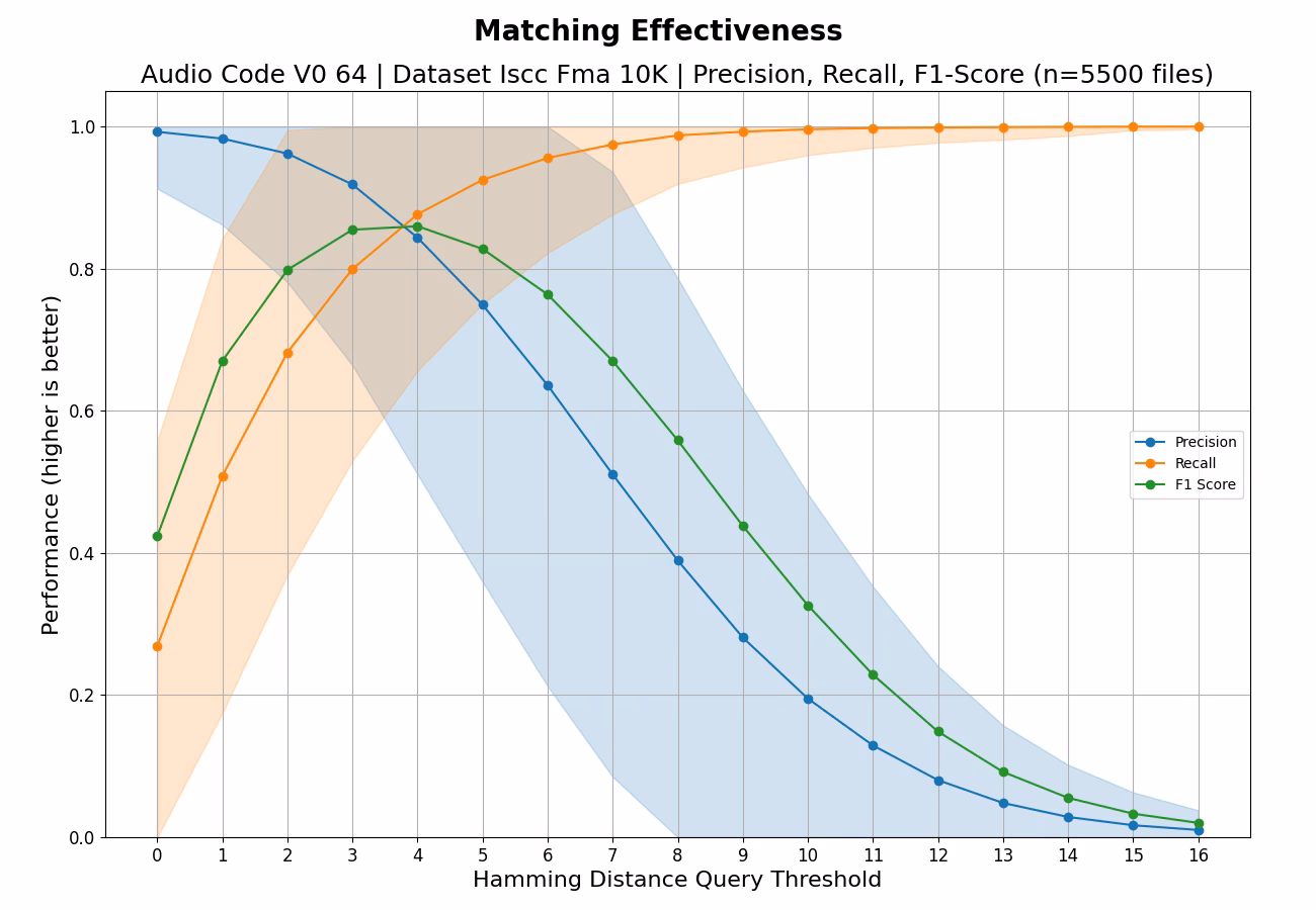
Effectiveness#
Understanding the Effectiveness Chart
This chart shows how well the algorithm finds matching files (like duplicates or near-duplicates) without making mistakes.
What the lines mean:
- Recall (orange): "Did we find all the matches?" A value of 1.0 means every match was found. Lower values mean some matches were missed.
- Precision (blue): "Are our matches correct?" A value of 1.0 means every reported match was real. Lower values mean some reported matches were wrong (false alarms).
- F1-Score (green): The overall balance between Recall and Precision. Higher is better. A perfect score of 1.0 means all matches were found with no false alarms.
What the shaded bands mean:
The colored bands around the Precision and Recall lines show the variation across different test queries. Narrow bands indicate consistent performance; wide bands suggest the algorithm works better on some files than others.
How to read the X-axis (threshold):
The threshold controls how "similar" two files must be to count as a match. Lower thresholds (left side) are stricter - only very similar files match. Higher thresholds (right side) are more lenient - somewhat different files can still match.
- Moving right typically increases Recall (find more matches) but decreases Precision (more false alarms).
- The best threshold depends on your use case: use lower thresholds when false alarms are costly, higher thresholds when missing matches is costly.
What makes a good result?
Look for the point where F1-Score peaks - this represents the best balance. An ideal algorithm would show high Recall and high Precision across all thresholds (lines staying near 1.0).
Robustness#
| Transformation | Minimum | Maximum | Mean | Median |
|---|---|---|---|---|
| compress-medium | 0 | 11 | 2.006 | 1.0 |
| echo | 0 | 15 | 3.598 | 3.0 |
| equalize | 0 | 12 | 1.214 | 1.0 |
| fade-8s-both | 0 | 4 | 0.436 | 0.0 |
| loudnorm | 0 | 5 | 0.55 | 0.0 |
| transcode-aac-32kbps | 0 | 10 | 1.786 | 1.0 |
| transcode-mp3-128kbps | 0 | 3 | 0.33 | 0.0 |
| transcode-ogg-64kbps | 0 | 7 | 0.864 | 1.0 |
| trim-1s-both | 0 | 5 | 0.936 | 1.0 |
| trim-5s-both | 0 | 11 | 2.4 | 2.0 |
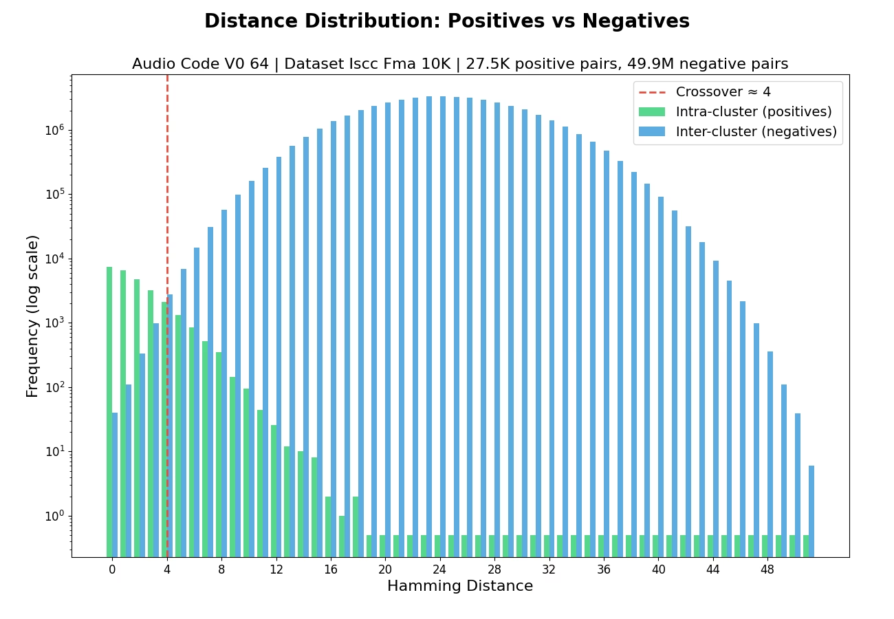
Distribution#
Understanding the Distribution Chart
This chart shows how the algorithm distinguishes between files that should match (duplicates) and files that should not match (different content).
What the bars mean:
- Green bars (Intra-cluster/Positives): Distances between files that ARE duplicates of each other. These should ideally be small (clustered on the left side).
- Blue bars (Inter-cluster/Negatives): Distances between files that are NOT duplicates. These should ideally be large (clustered on the right side).
Why separation matters:
A good algorithm creates clear separation between green and blue bars - duplicates have small distances, non-duplicates have large distances. This makes it easy to set a threshold that correctly identifies matches.
The crossover point (red dashed line):
If shown, this marks where the distributions overlap - the distance at which you start seeing more non-duplicates than duplicates. Setting your matching threshold near this point balances finding matches against avoiding false alarms.
What makes a good result?
- Green bars concentrated on the left (low distances for duplicates)
- Blue bars concentrated on the right (high distances for non-duplicates)
- Minimal overlap between the two distributions
- A late crossover point (further right is better)
Performance#
Throughput Statistics
| Metric | Value |
|---|---|
| Minimum | 0.3354 MB/s |
| Maximum | 25.1377 MB/s |
| Mean | 5.2704 MB/s |
| Median | 4.5754 MB/s |